merTools 1.0: prediction intervals for mixed models, validated against brms

After a decade on CRAN, merTools 1.0.0 is out today. It has been a long-term goal of mine to bring merTools to a stable state, fix outstanding bugs, and rework the `predictInterval()` function at its core to be more modular and easy to maintain. This release achieves that and marks the package as feature complete and the start of a long-term-support (LTS) phase. This release hits the goal of 1.0.0 of a stable API, outstanding issues closed, a correctness fix at the core of predictInterval(), and modularity in the core prediction interval functionality. The documentation is also now available [via a pkgdown site as well!](https://jknowles.github.io/merTools)

install.packages("merTools")

What merTools is for #

merTools has been on CRAN since 2015, with over 457,000 downloads and about 8,000 a month. It exists to get the most out of large mixed-effects models fit with lme4 . Its headline function, predictInterval(), produces prediction intervals for lmer/glmer models by simulating from the joint distribution of the fixed and random effects — the approach from Gelman and Hill (2007),¹ the same machinery behind arm::sim().

The motivation is practical. lme4::bootMer() and full MCMC give you principled uncertainty, but on models with tens of thousands of groups they can be impractical or simply too slow to use interactively.

predictInterval() is built to give you honest intervals on exactly those models, in about a second.

Try it out and validate it against brms! #

The obvious question for a simulation-based approximation is how close it is to doing the full Bayesian thing. When we first wrote merTools brms was in its infancy, but since then it has become my go-to for most Bayesian inference and, frankly, made much of merTools obsolete. I used an LLM to assist me with refactoring the code and responding to open issues, so I wanted to create a new set of tests and benchmarks to validate that the package still worked.

So for 1.0 I created a new short vignette that compares brms and merTools results side by side: the same data and the same model — the bundled hsb data (7,185 students in 160 schools), modeling math achievement from student SES, school-mean SES, and a school-varying SES slope. We hold out 20% of students to test on.

data(hsb)
hsb$schid <- factor(hsb$schid)
new_schools <- sample(levels(hsb$schid), 6)
hsb$.set <- "train"
hsb$.set[hsb$schid %in% new_schools] <- "test_new"
seen <- which(hsb$.set == "train")
hsb$.set[sample(seen, round(0.2 * length(seen)))] <- "test_seen"
train     <- droplevels(hsb[hsb$.set == "train", ])
test_seen <- hsb[hsb$.set == "test_seen" & hsb$schid %in% levels(train$schid), ]

f1 <- mathach ~ ses + meanses + (ses | schid)
m_lme <- lmer(f1, data = train)

# Fit brms once and cache it. Persist the genuine from-scratch fit time to a
# file, so the timing table below reports the real compile+sample cost even on
# later renders that just read the cached fit (which take ~2s, not ~7 min).
brms_cache <- file.path(outdir, "brms_hsb_meanses.rds")
time_cache <- file.path(outdir, "brms_hsb_meanses_seconds.rds")
fresh_fit <- !file.exists(brms_cache)
elapsed <- system.time(
  m_brm <- fit_brm(f1, train, gaussian(), "brms_hsb_meanses"))[["elapsed"]]
if (fresh_fit) saveRDS(elapsed, time_cache)
brms_fit_seconds <- if (file.exists(time_cache)) readRDS(time_cache) else elapsed

Point estimates are essentially identical #

Both methods condition on the same estimated fixed effects and school BLUPs, so the conditional-mean predictions agree almost exactly.

lme_mean <- predict(m_lme, newdata = test_seen)
brm_mean <- colMeans(posterior_epred(m_brm, newdata = test_seen, allow_new_levels = TRUE))
c(correlation = cor(lme_mean, brm_mean),
  mean_abs_diff = mean(abs(lme_mean - brm_mean)),
  response_sd = sd(test_seen$mathach))

#>   correlation mean_abs_diff   response_sd 
#>    0.99984045    0.03670134    6.71745425

ggplot(data.frame(merTools = lme_mean, brms = brm_mean), aes(merTools, brms)) +
  geom_abline(slope = 1, intercept = 0, linetype = 2, color = "grey50") +
  geom_point(alpha = 0.3, size = 0.8, color = "#1B9E77") + coord_equal() +
  labs(x = "lme4 predict()", y = "brms posterior_epred()") +
  theme_civilytics()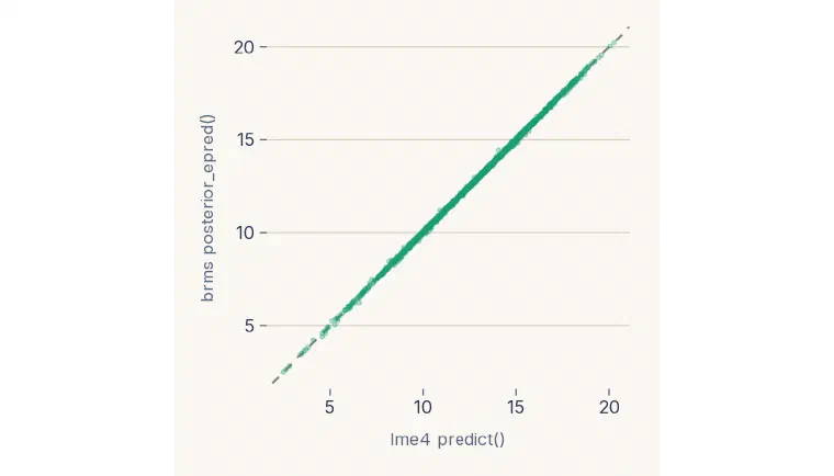

And they are equally well calibrated #

The real test is out-of-sample: do nominal intervals cover held-out scores at the nominal rate? We draw a full predictive distribution for each held-out student from each method — predictInterval(returnSims = TRUE) and brms::posterior_predict() — and compare empirical coverage. Both track the nominal level, and each other.

The mt_draws() helper used below — saved alongside the analysis — just wraps predictInterval() to hand back the raw simulation matrix:

# One column of posterior-style draws per row of `newdata`.
mt_draws <- function(fit, newdata, ...) {
  pi <- predictInterval(fit, newdata = newdata, returnSims = TRUE, ...)
  attr(pi, "sim.results")
}

mt_seen <- mt_draws(m_lme, test_seen)
pp_seen <- posterior_predict(m_brm, newdata = test_seen, allow_new_levels = TRUE)
data.frame(nominal = NOMINAL,
           merTools = coverage(mt_seen, test_seen$mathach, NOMINAL),
           brms     = coverage(pp_seen, test_seen$mathach, NOMINAL))

#>   nominal  merTools      brms
#> 1    0.50 0.4569776 0.4598698
#> 2    0.80 0.7895879 0.7932032
#> 3    0.90 0.9168474 0.9168474
#> 4    0.95 0.9660159 0.9703543

At a fraction of the cost #

t_lme <- system.time(lmer(f1, data = train))[["elapsed"]]
t_mt  <- system.time(mt_draws(m_lme, test_seen))[["elapsed"]]
t_pp  <- system.time(posterior_predict(m_brm, newdata = test_seen,
                                       allow_new_levels = TRUE))[["elapsed"]]
data.frame(
  step = c("lme4 fit", "predictInterval", "brms fit (compile+sample)", "posterior_predict"),
  seconds = round(c(t_lme, t_mt, brms_fit_seconds, t_pp), 2))

#>                        step seconds
#> 1                  lme4 fit    0.07
#> 2           predictInterval    0.66
#> 3 brms fit (compile+sample)  409.13
#> 4         posterior_predict    2.38

The entire lme4 + predictInterval() path runs in about a second; the single brms fit takes several minutes — a couple of orders of magnitude, and the gap only widens on the large models predictInterval() was really built for. The point isn’t to stop using brms: if you want the full posterior, use it. The point is that when full MCMC is impractical, predictInterval() is a fast, well-calibrated stand-in. The full story — new-group handling and a binomial GLMM — is in the validation vignette .

When full MCMC is impractical, predictInterval() is a fast, well-calibrated stand-in.

Visualizing group effects with plotREimpact() #

New in 1.0, plotREimpact() visualizes REimpact() output — the fitted outcome across the distribution of a grouping factor’s effect. Pass a named list and it overlays grouping factors on shared axes, so you can compare their influence directly. Here, the instructor and student effects in the InstEval ratings data:

m1 <- lmer(y ~ service + lectage + studage + (1 | d) + (1 | s), data = InstEval)
imp_d <- REimpact(m1, InstEval[7, ], groupFctr = "d", breaks = 5, n.sims = 300, level = 0.9)
imp_s <- REimpact(m1, InstEval[7, ], groupFctr = "s", breaks = 5, n.sims = 300, level = 0.9)
plotREimpact(list("Instructor (d)" = imp_d, "Student (s)" = imp_s)) + theme_civilytics()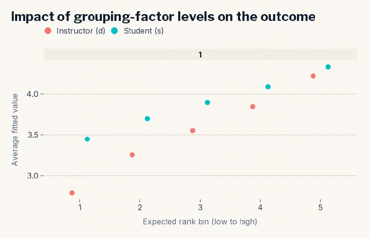

Moving a case from the bottom to the top of the instructor-effect distribution shifts the predicted rating substantially more than the same move across the student distribution — the instructor grouping factor carries more of the signal.

What else is new in 1.0 #

The release notes have the full list; the highlights:

• Correctness fix for nested random effects (#124). predictInterval() was returning seed-dependent point estimates when a prediction frame mixed observed and unobserved levels of an interaction grouping factor (e.g. (1 | a/b)). A max.col() tie-break was silently letting an unobserved level borrow a random observed level’s effect. Unobserved levels now correctly fall back to the fixed effects; observed-level predictions are bit-for-bit unchanged.

• New new.levels = "draw". For a group the model never saw, the default ("zero") drops its random effect; "draw" instead samples the effect from the estimated random-effect covariance — the direct analogue of brms::posterior_predict(allow_new_levels = TRUE). The default is unchanged.

• plotFEsim() now highlights significant terms, and shinyMer() is revived and extended with a Model Summary tab and subset-based draws.

Why LTS / maintenance mode #

merTools does what it set out to do, and the API has been stable for years. Going forward, 1.0.x releases will be about keeping it healthy — bug fixes, CRAN and dependency compatibility, and documentation — rather than churning the interface.

Get it / cite it / file issues #

install.packages("merTools")
citation("merTools")

• Package site & vignettes: https://jknowles.github.io/merTools/
• Source & issues: https://github.com/jknowles/merTools

Thanks to everyone who has contributed over the years — Carl Frederick, Alex Whitworth, Ben Bolker (@bbolker), Davis Vaughan (@DavisVaughan) — and to the issue reporters who made this release better, including @dotPiano, whose report led to the #124 correctness fix.

References #